Coding "This is Us"
About 6 months ago, we presented a PC demo production at Revision 2025. If you haven’t seen it yet, go watch it here. 🙂
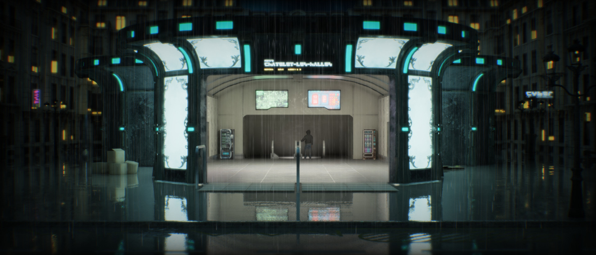
Shot from the intro sequence of This is Us.
In this post, I thought I’d go through some of the graphics techniques that were showcased in the release and that I think are exciting.
Path tracing
Arguably, this is the biggest one. 🙂
One thing to keep in mind though is that the engine used here is still based on OpenGL, which means that hardware-accelerated ray tracing isn’t an option… (at least not until someone makes an extension for it, akin to the recently merged mesh shaders extension) Not a big issue in practice, as the engine supports since its inception (circa 2015-16) an acceleration structure for ray/triangle intersection loosely based on this reference initially, although later extended to irregular grids.
So, this calls for a somewhat different thinking from the current path tracing developments that can be seen in games for instance. Specifically, the ray count really should be kept as low as possible, so that the framerate can remain at 60Hz…
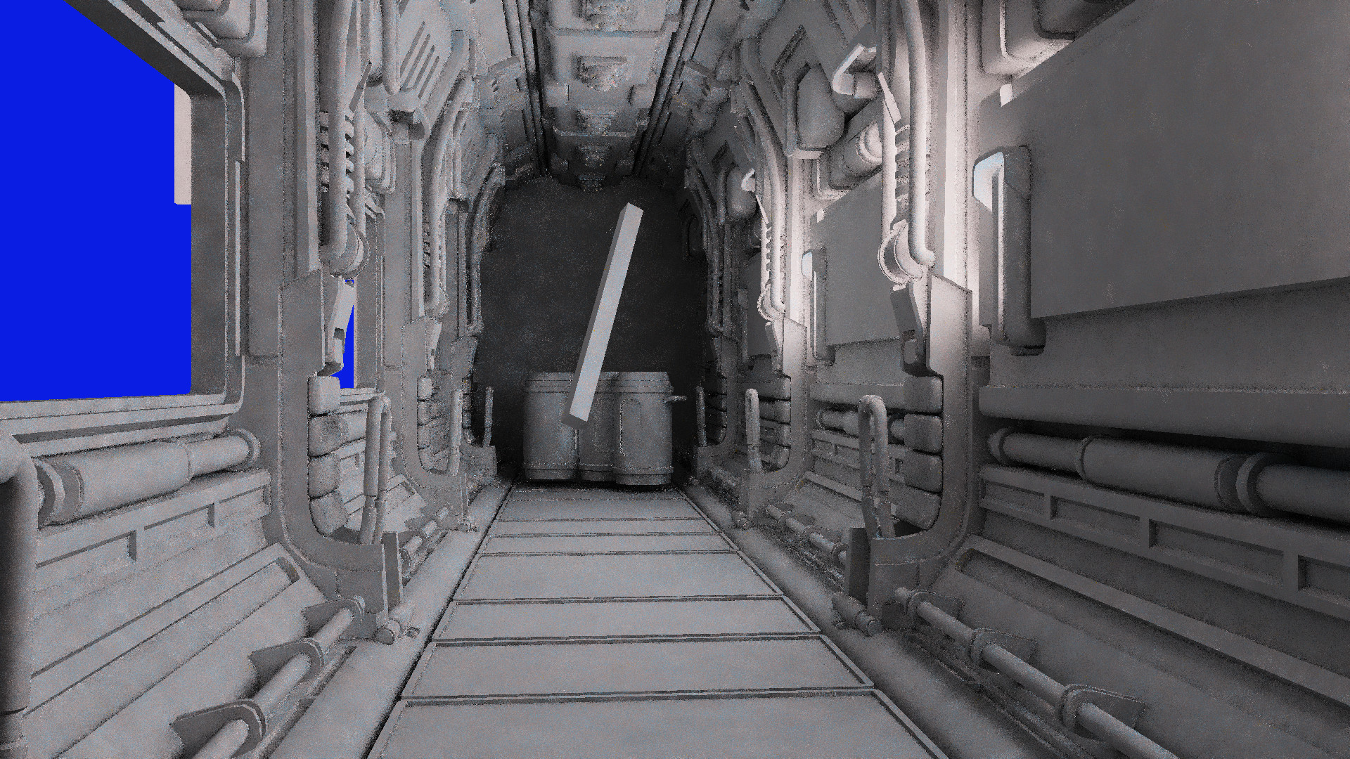
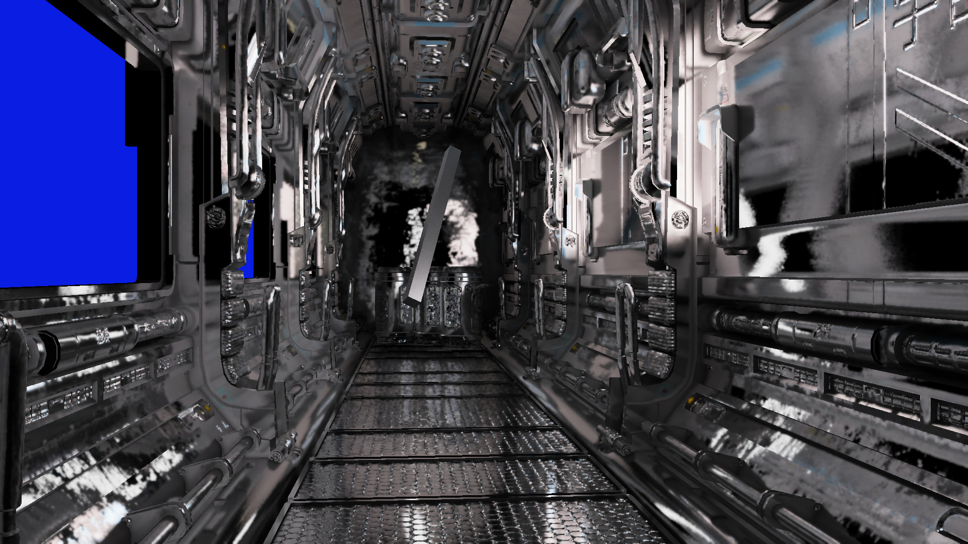
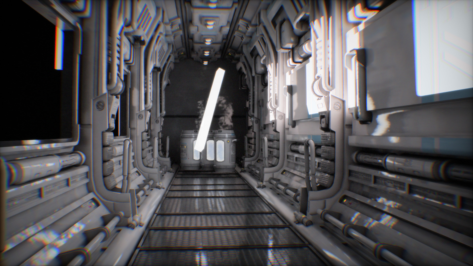
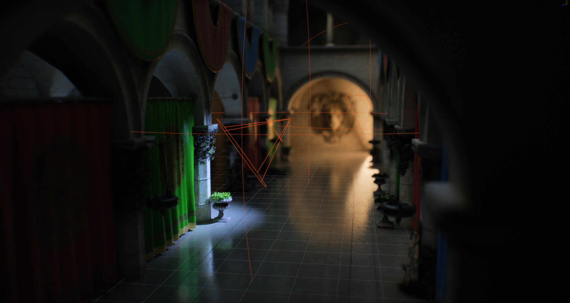 The path tracer in action inside the timeless “Sponza” scene.
… which is a bit of a challenge when tackling path tracing. In short, path tracing requires you to make a random choice every time you hit a surface, explore the direction resulting from that random choice (using ray tracing), only to then repeat these same steps on the next hit. Not only does this typically equate to lots of expensive rays being cast, but the result is also generally unusably noisy. 😕
Enters radiance caching.
The idea behind radiance caching is to terminate the paths early into a data structure that approximates the scene’s lighting. Not only is the performance improved due to the traces being shallower, but the noise is also greatly reduced thanks to the filtering offered by the data structure.
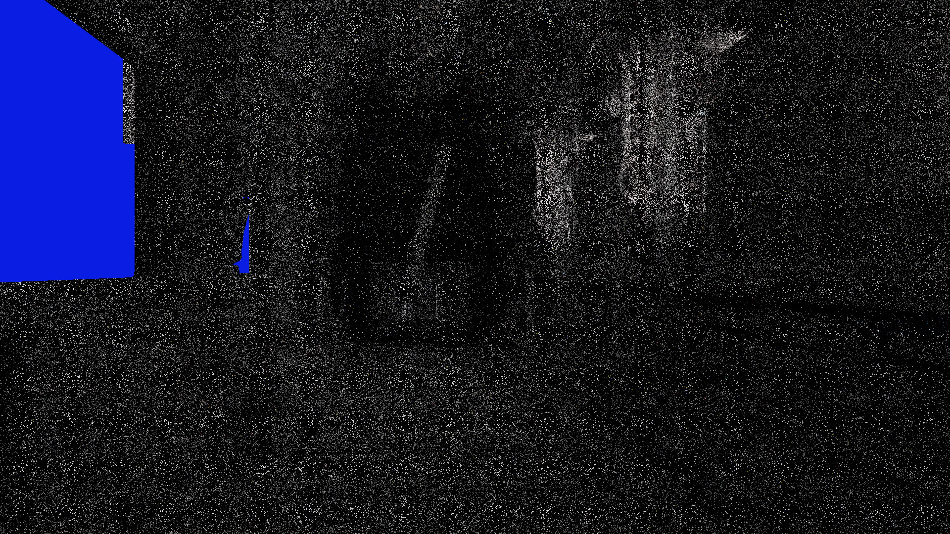
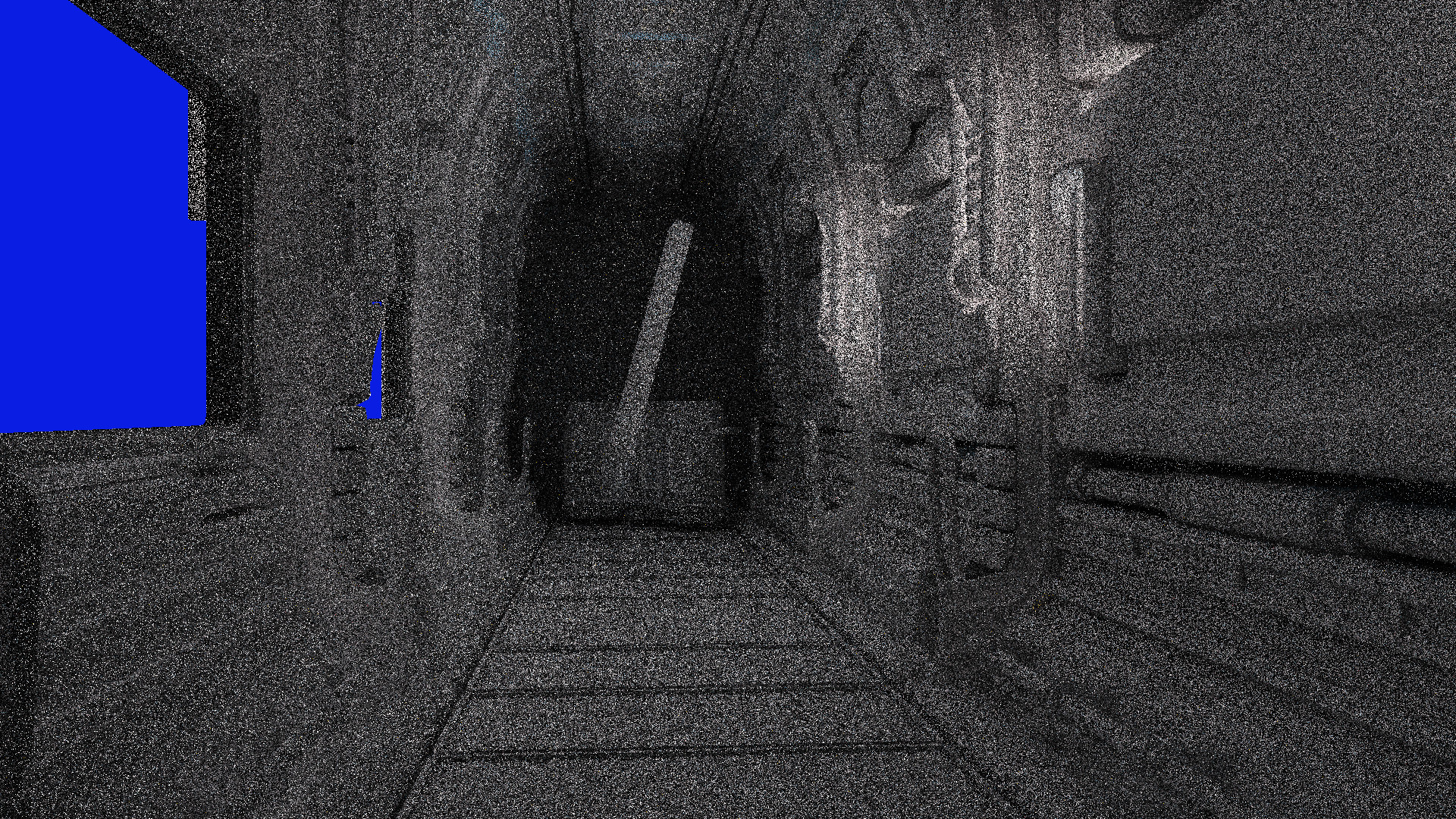
Test renders without and with radiance caching.
Here, we’ll be using spatial hashing to generate the structure, and the update is as follows:
- Once a frame, go through all the cells (initially, there are none) and check whether the decay has completed; evict as required.
- Every time the cache is looked up, do the following:
- Hash the position and normal at the hit point to build a list of affected cells (these may be new cells). Make sure to reset the decay back to its original value. (If the cell was already estimated this frame, we can exit here, without adding it to the list.)
- Pick a hit point at random for every cell in the list; we’ll use it for computing the direct lighting contribution for the cell as well as for spawning a “bounce ray” (using cosine-weighted sampling for instance).
- Whatever the bounce ray hits, check whether a cell exists; if so, use its radiance as contribution, if not, do nothing.
uint SpatialHash_FindOrInsert(float3 position, float3 normal, float hitDistance)
{
    // Inputs to hashing
    int3 p = floor(position / g_CellSize); // cell size can be made adaptive for LOD support
    int3 n = clamp(floor((0.5 * normal + 0.5) * 4.0), 0.0, 3.0);
    int  b = (hitDistance < g_CellSize ? 1 : 0); // light leak heuristic

    // https://www.shadertoy.com/view/XlGcRh
    uint bucketIndex = pcg(p.x + pcg(p.y + pcg(p.z + pcg(n.x + pcg(n.y + pcg(n.z + pcg(b)))))));
    bucketIndex %= g_BucketCount; // map to cell bucket
    uint checksum = xxhash32(p.x + xxhash32(p.y + xxhash32(p.z + xxhash32(n.x + xxhash32(n.y + xxhash32(n.z + xxhash32(b)))))));
    checksum = max(checksum, 1); // 0 is reserved for available cells

    // Update data structure
    for(uint i = 0; i < g_BucketSize; i++)
    {
        uint cellIndex = i + bucketIndex * g_BucketSize;
        uint cmp       = atomicCompSwap(hash[cellIndex], 0, checksum);

        if(cmp == 0)
            return cellIndex; // inserted a new cell
        if(cmp == checksum)
            return cellIndex; // found an existing cell
    }

    return 0xFFFFFFFFu; // out of memory :'(
}
A great property of this approach is that we only trace one “bounce ray” per affected cell, while still getting a decent approximation of “infinite” multiple bounces (temporally recurrent, in fact). This turns out to be a great knob for balancing quality vs. performance. Indeed, using smaller cells, we achieve greater fidelity but at higher cost. Conversely with larger cells, we introduce more bias, but our path tracer now runs much faster. This property can easily be tweaked on a per-scene basis to obtain the best possible results. 🙂
Still, the image remains fairly noisy.
The second technique we’ll employ here is known as ReSTIR (short for “Resampled Spatio-Temporal Importance Resampling”). And specifically, the “GI” variant of it.
Test renders without and with ReSTIR.
Covering the depths and details of ReSTIR would make for a post of its own, so suffice to say that the approach chosen here, unsurprisingly, aims at minimizing the number of rays being cast.
A cool trick for this was proposed by the folks over at Traverse Research. They pointed out that one could simply retrieve an AO mask (short for “Ambient Occlusion”) from the initial ray trace. This mask wouldn’t be applied to the lighting directly, as is usually the case with AO, but rather used for weighing the validity of combining reservoirs. If the reservoirs’ AO values match closely, the probability of combining them increases, otherwise, it is reduced. This greatly improves preservation of contact shadows and details, at no additional ray tracing cost. 🙂
Finally, the image is cleaned up using some standard spatiotemporal denoising. The denoiser itself is fairly simple (and fast); use temporal reprojection when possible, fall back to spatial filtering when not. The number of accumulated temporal samples is stored in the alpha channel and is used to “fade away” the amount of spatial filtering as history becomes more reliable.

Denoised diffuse and specular signals.
A quick word on specular; it uses about the same data flow than diffuse but with a few additional dedicated heuristics. Specifically, “BRDF-based ratio estimator” by Tomasz Stachowiak is used for upscaling the signal (the path tracer typically renders at ¼ spp, or even ⅛ spp at times…), while “dual-source reprojection” (by the same author) ensures that smooth surfaces are reprojected (more or less) correctly.
 The composited image… finally!
Fluid simulation
This is an area I’ve been wanting to dive further into for quite some time. While there’s still a lot more to explore for me (hopefully in some not-so-distant future production…), I’m quite happy with what we’ve been able to show back in April.
The setup I ended up with is mostly inspired by this post from Morten Vassvik. The idea is to pre-fetch the neighboring data efficiently into LDS (short for “Local Data Share”) by having all lanes cooperate to the operation. We can then synchronize the group and perform our computations with the neighboring cells’ information close by and ready for fast access. 🙂
In my scenario however, I was interested in dealing with particles and implementing smoothed-particle hydrodynamics, or SPH for short. So, I went ahead and started binning the particles into tiles of 4x4x4 cells. The tiles themselves are sparsely allocated using… spatial hashing, again! A very useful technique for sure.
As part of the build process, I also generate a list of all the tiles in the structure. My initial idea was to then dispatch one 4x4x4 group per tile for the solver, but due to the vastly varying number of particles in each cell, the performance was terrible…
 Some early test of the tiled SPH approach using ½ million particles.
So instead, I divided each tile into a list of subtiles; for instance, a tile with 150 particles in it gets broken down into two subtiles of 64 particles and one subtile of 22, or three subtiles in total. All that’s needed for addressing the subtiles is the tile index and corresponding subtile index (all packed into a single 32-bit integer in my case). I can now dispatch over all subtiles and go much more wide and even across the device. 🙂
At the start of the shader, we then begin with performing the pre-fetching of the neighboring particle lists into a 6x6x6 multidimensional LDS array as well as picking the particles linearly based on the subtile index. From that point on, SPH can run pretty much unmodified from a regular implementation processing one particle per lane, but with much better performance.
The final step on the fluid journey was meshing, that is, generating a list of triangles modelling the isosurface implicitly represented by the particles. For this purpose, my plan was to use the Marching cubes algorithm. But in order to run the algorithm, we must first derive a field from our set of particles…
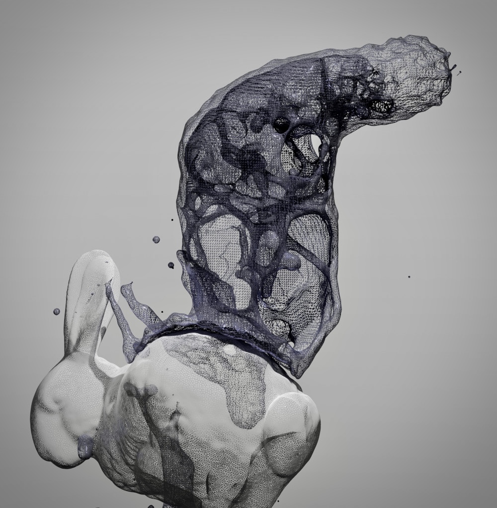 Some Marching cube’d fluid thrown onto the Stanford bunny.
I ended up using the exact same data structure that the one used for the SPH simulation, but this time I subdivided each cell further into either a 2x2x2 or 4x4x4 subdivision (left as a tweakable option of the algorithm). For each of the subcells, all we need to do is compute the field value using a routine very similar to the SPH density pass (although running at the subcell level) as well as the partial derivatives in all X, Y, and Z directions (these can be used to derive smooth normals at each generated vertex). One additional thing to perform however is a dilation of the data structure by at least one cell, as the resulting surface may generate triangles outside the regions directly occupied by the particles. This is done efficiently as a pre-pass to estimating the field.
Finally, Marching cubes is run over the computed field, and a bit of smoothing is applied by simply moving the vertices by a small amount in the opposite of the normal direction, which helps the resulting mesh look sharper and slightly more fluidlike.
One last thing
This post is pretty long already but I thought I’d still briefly mention how the lighting (or shadows rather) is computed for the particles. A commonly used technique for shadowing particle systems is known as Deep Opacity Maps. These essentially extend traditional shadow maps with depth slices to handle the volumetric nature of the shadowing (required due to our particles being slightly transparent rather than fully opaque).
In my case however, I want to be able to handle multiple light sources, which would require drawing multiple deep opacity maps (once for each light effectively), and envision eventually connecting the particles’ lighting system to the path tracer described earlier. So, instead of dealing with each light individually, I’d rather create a single acceleration structure, which I could then use for all lights and, in the future, indirect lighting.
I named this new data structure “particle volume” although in effect, all it really is, is a 3-dimensional density field…
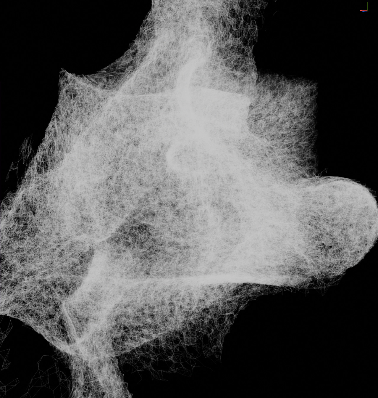
From left to right: no lighting, particle volume, shadowed particles.
We could imagine using a similar spatial hashing setup to the one used for our fluid simulation. However this time, we’ll want to traverse the grid cells many times and in many different directions (a technique known as ray marching). So spatial hashing isn’t a good fit here, as the overhead of accessing each visited cell would simply kill the performance.
Instead, the new data structure should encompass the whole particle system’s bounding box (estimated dynamically using 6 min/max parallel reductions); we’d then advance the ray to the intersected edge of the box (if the ray started outside of the volume that is) and simply march through the cells from that point on, accumulating the amount of “matter” encountered on the way to derive the final opacity value.
As for the data structure itself, I decided to still go with a sparse approach, again using tiles made of 4x4x4 cells. This time though, the buffer storing the tiles is allocated in full by accounting for the worst-case scenario. The resulting memory requirements remain modest however, as all we really need to represent a tile is a single integer value; this property is in turn used as a “pointer” into the underlying (sparse) cell storage.
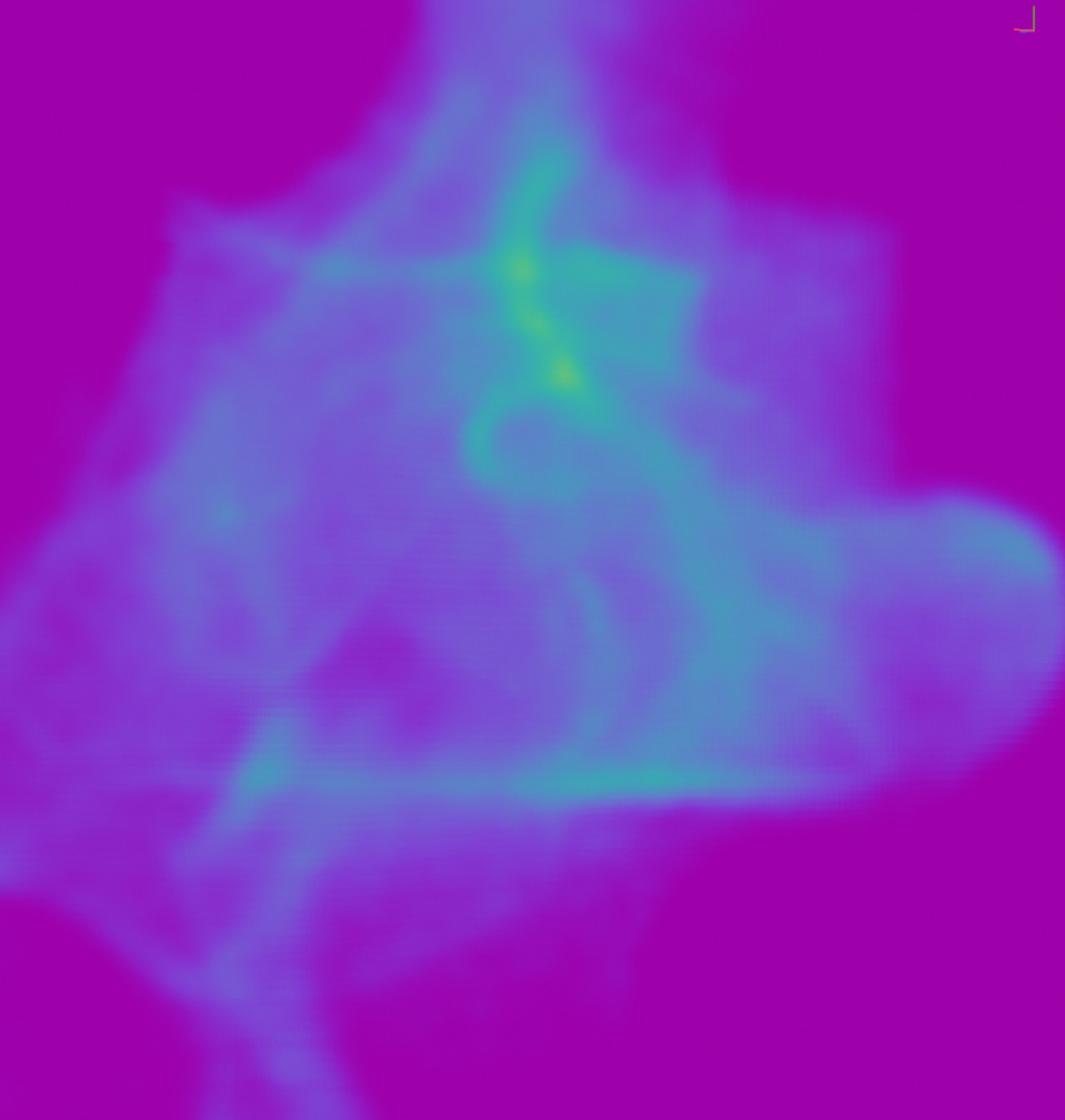
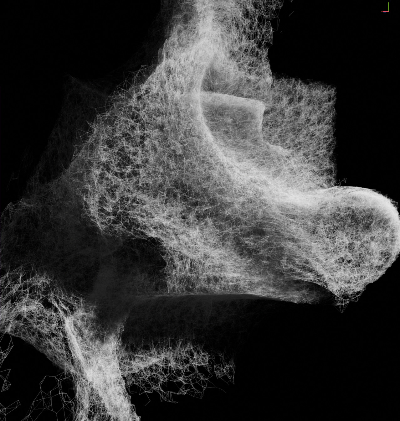
Once the cells’ allocation has completed, a per-cell counter is atomically incremented for each particle that falls into it. This alone would result in fairly aliased shadows, so the build finishes with a 3-dimensional separated blur pass using the tile size as radius, allowing to make it pretty fast (we only need to look up one tile to the left and one to the right) while smoothing out the lighting.
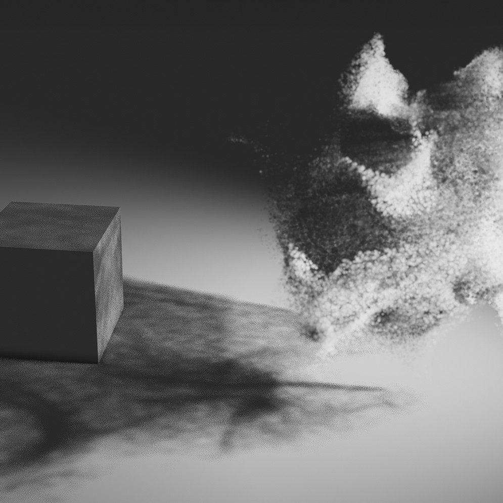
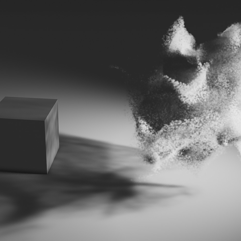
Without vs. with blurring the density field.
Finally, the data structure is traversed, starting from each particle and towards every targeted light to achieve self-shadowing on the system itself. Then we run the same process, but starting from every pixel inside the depth buffer, allowing for particles to cast shadows onto the scene’s geometry. Additionally, we can further use our shadow maps during particle tracing to get geometry casting shadows back onto the particles themselves. We then end up with a pretty complete and unified shadowing system. 🙂
Conclusion
If you’ve made it this far, congratulations!
If not, I hope that you nevertheless found some of the information in this post to be useful and/or inspiring. As for myself, I feel I am just getting started, so watch this space.
comments powered by Disqus